Estimating cost-effectiveness for problems of unknown difficulty

Owen Cotton-Barratt

This is part of a series of posts on how we should prioritise research and similar activities. In a previous post we explored how we should form subjective probabilities about chances of success of problems of unknown difficulty. This post is concerned with how to use these probabilities to estimate the expected value of working on such problems. This is related to the question of how to estimate the expected value of working in a research field, which I addressed at the end of this post. A key aspect of both questions is the need to compare what we expect to happen in the counterfactuals where we make extra investment in the problem or don’t do so.

Counterfactual benefits

In order to prioritise between different options, it’s useful to understand the short-term impact of different paths, but this isn’t sufficient. We want to understand as much as possible about the longer-term effects of different routes.

This is quite salient in the case of knowledge problems. Once solved, they usually provide benefits not just once, but in a continuing stream into the future whenever anyone uses the output. If we want to calculate the true benefit of doing the work, we should try to model what the differences will be if we don’t do the work. Generally that will mean not that the work doesn’t occur, but that it isn’t done until later.

Of course this doesn’t always apply. Perhaps we are trying to break a cypher to de-encrypt one message, and we don’t foresee the techniques being useful again. In this case we should make a more straightforward model of the effects. But the dynamic of solving a problem providing a stream of benefits is common, so we analyse it here. Again, this is a crude model, so the answer it gives is likely to be useful as a starting point or order of magnitude rather than an accurate and precise figure.

Single funder case

We’ll first explore the case where you are, and expect to be, the only funder for the research. This could apply if it’s a specialised problem; it also gives the appropriate perspective for societal benefits and costs.

Assumptions: We’ll compare between doing extra research today, and saving the resources for a year and doing the research then. We want a couple of assumptions here:

• That we can freely move research from today to tomorrow. This can often fail to be exactly true, because labour is less flexible than money, but it seems reasonable as a first approximation.

• That the overall desirability of doing extra research at different times is a concave function with time. This means that to check whether it’s best to do research today we need only check whether today is a local maximum, rather than comparing to all possible future points. In cases where the research is generating constant benefit each year, or a benefit scaling with the size of the economy, this should be true.

Given these assumptions, compare the counterfactuals where we invest 1 extra dollar of resources in research today, versus hold onto the money for a year and invest the resources then. Under our model we see the following benefits:

Here a represents the extra chance of success this year from investing the resources. The value i represents the real interest rate earned (properly it should also incorporate the changing cost of research, if this is believed to be non-zero). So we face a tradeoff between getting interest by investing for sure, and a chance of getting a solution a year earlier. In each case the total amount of research done by the end of next year is the same, so for the purposes of the comparison what happens after that point can be ignored.

Assume that the marginal chance is given by a = k/z, where z is the total resources invested so far and k is a constant (thus fitting the form we discussed in previous posts). Then if B is the benefit to us of having a solution this year rather than next, the benefit of research now will be kB/z; the benefit of research later will be i.

At the optimal level of investment in research, the marginal value of investing extra resources into research today will be zero. This occurs when z = kB/i.

If we assume that i = 3%, and that k = 1/15 (corresponding for example to the box model and a belief that we have at least a half chance of finding a solution before we have done a thousand times as much research as we have today), then the total spending to date should be approximately twice the benefit that would be produced in a year. If we think we are likely (⅔ chance) to get a solution with a hundred times as much research we already have, the total spending to date should be about four times the benefit expected in a year.

If B grows over time at the same rate i (which may be plausible for some discoveries which would have a multiplicative benefit to the economy), and we aresmoothly increasing the annual funding, then the annual spending should be around Bk.

In reality it can be hard to be in this case, because not all of the resources are monetary. There is a pool of labour willing to work on the problem that you will draw upon, and there may be other exogenous drivers.

Relation to the three-factor model for cause selection

GiveWell and 80,000 Hours have used an informal ‘three-factor model’ for selecting causes. They evaluate causes by their scale, their neglectedness, and their tractability.

One way to think of working on a cause is as working on a problem of unknown difficulty. This doesn’t apply to all work; some — such as distributing insecticide treated bednets against malaria — is more of the form of scaling up interventions of (approximately) known cost-effectiveness. But for several causes we might hope to find a solution that will enable the whole problem, or a substantial fraction of it, to be dealt with once and for all. This could include looking for a vaccine for malaria, or other more speculative causes.

Our model for the benefit of immediate investment said that the benefit was of size kB/z. The three terms here line up pretty well with the components of the three factor model. The scale of the problem is expressed by B, the size of the benefit. The neglectedness gives us the term 1/z, the reciprocal of the amount of investment so far. And the remaining term, k, measures the tractability of the problem.

We did not set out to reproduce the three-factor model. That we have arrived at a formal model very similar to it provides some evidence for the robustness of the three factor model, and provides a natural more formal interpretation of the factors. While it was always fairly easy to see how you’d likely cash out scale and neglectedness, it wasn’t at all clear how to put a numerical value on tractability. It could be useful that this gives us a way.

Are there any lessons to be drawn from this? One is that tractability may matter less than the other two factors. Under the box model discussed, we have k*= p/(ln(y/z)), where y is some level of resources such that we believe there is a probability p of success by the time y resources are invested. We might like to consider k = θk*, where θ is a factor to adjust for deviation from the box model. Then k itself decomposes into three factors: p, the likelihood of eventual success; 1/(ln(y/z)), which tracks time we may have to wait until success; and θ, which expresses something of whether we are currently in a range where success is at all plausible.

If the problem is something that we believe is likely to be outright impossible, like constructing a perpetual motion machine, then p will be very small and this will kill the tractability. If the problem is necessarily hard and not solvable soon, like sending people to other stars, then the box model will be badly wrong (or is best applied with our current position not even in the box), so θ can kill the tractability. But if it’s plausible that the problem is soluble, and it might be easy — even if might also be extremely hard — the remaining component of tractability is 1/(ln(y/z)). Because of the logarithm in this expression, it is hard for it to affect the final answer by more than an order of magnitude or so.

It is fortunate for our endeavour of estimating cost-effectiveness that the tractability does not play too large a role. This is because while it can often be a tricky empirical question to estimate the neglectedness, and a trickier speculative question to estimate the scale of benefits, there is much more guesswork still involved in saying how much more work might be needed to solve a problem. But because it is transformed by a logarithm, innaccuracy in this part of the estimation will not affect the final answer by very much.

I’ve considered the analogies with the three-factor model in the context of the single-funder scenario because the answer produced was simple and easy to analyse. However it is not generally the right perspective for those choosing causes. In the next section I’ll investigate how the cost-effectiveness estimates should change when we take a different perspective, and ask how much that changes the link with the three-factor model.

External funding case

We’ll now consider the case where there are other people investing resources into the problem, where you may care less about their resources than your own.

A useful simplifying assumption is:

Unresponsive funding: Future resource inputs from other sources will be unaffected by our decisions (until the problem is solved).

This could in general fail in either direction. Work in an area can demonstrate to others that the area is worthwhile, and attract extra resources. On the other hand others might respond to the diminishing marginal opportunities by putting in less. For calculating the true counterfactual impact it is relevant to us not just how much the eventual shift in funding is, but when that occurs: funding earlier is generally better, because of the chance of generating the research benefits for longer.

It seems likely that in the very short term, extra resources will not change inputs from others. In the medium term you might or might not attract extra resources to the area. And in the long term perhaps you would displace extra funding, as other funders adjust for the reduced marginal benefit available as a result of your resources. For now I propose to use the unresponsive funding assumption as I believe it will be approximately correct, but a more complicated regime could certainly be modelled, and I am very interested in returning to this question and searching for data or other insights.

The benefit of marginal resources put into the problem today comes in two forms: first, the benefit gained by moving the solution forwards in time; second, the resources which would have finished solving the problem but now can be used for something else. To estimate the value of these we should model when the solution is likely to be found. This makes the external funding case more complicated than the single funder case, because we need to make some assumptions about the rate of resources allocated to it over time, as well as about the difficulty of the problem.

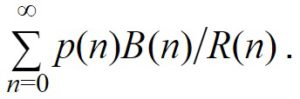
Assume that in year n the resources allocated will be R(n). We’ll consider the impact of investing an extra dollar now. If the solution would be found in year n, then we will move forward the solution by 1/R(n) years. If B(n) is the net present value of the benefit generated by a solution in year n, this means that if we would solve the problem in year n, the benefit from an earlier discovery will be B(n)/R(n).

Letting p(n) be the probability of discovery in year n, we have the expected value from earlier discovery is given by:

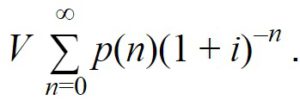
If a solution is found in year n, the extra invested dollar will be displaced and freed up for another use. The net present value of this will be 1/(1+i)^n, where i is the interest rate. To compute the value to us, we may wish to multiply this by an additional factor V, representing the fact that the resources will be held by others (for example if we are considering investing in a malaria vaccine, we may think that any displaced funding is likely to go into useful projects, but perhaps not as useful as we could have found, and use V = 0.8). Then the expected value from displaced resources is given by:

To find the total counterfactual value of investing now we can sum these two expressions. As a reminder, so far we’ve assumed:

1. Funding is unresponsive to our investment.

2. The solution arrives all at once.

3. The value of the solution in a given year doesn’t depend on how long the solution has been held for.

To further simplify and allow easier calculations, we’re going to add in assumptions about the distribution of possible difficulties of the problem, and what future growth of resources working on the problem looks like. If for a specific problem you have good data available, that might be preferable to using the following assumptions.

4. Funding on the problem has been growing exponentially and will continue to do so, at a constant rate f per year. So R(n) = (1+f)^R(0).

5. Problem difficulty is distributed as in the box model, i.e. uniformly between present total spend z and some upper limit y.

6. The net present value of the benefit is the same in every year. i.e. B(n) = B is constant. This is plausible if the discovery provides a multiplicative effect on the economy, so its value grows to cancel out the discount rate.

Assumption (4) will usually hold approximately because the economy grows roughly exponentially and the share devoted to a given problem has a growth behaviour too. If the current annual spend is R(0), and the growth rate is f of resources is f, the total spend z so far is given by:

z = R(0)/(1-(1/(1+f))).

When f is small, this is well-approximated by the simpler: z = R(0)/f. Note that a consequence of (4) is that the total-spending-to-date is growing at the same exponential rate f as the annual spending.

If we use the box model (5) while assuming exponentially growing funding (4), then before total funding reaches y (i.e. until we reach the end of the box), the annual chance of success is constant. So we have p(n) = k, for n < a threshold N, and 0 for n ≥ N (assuming for simplicity that the end of the box comes at the end of a year; a continuous version of this analysis might be more natural and in practice I’m making several assumptions which hold exactly in the continuous version). To find N we need to find the time when the total resources invested equal y. This is when the resources have increased by a factor of y/z, so N = log(y/z)/log(1+f). If the probability of success by the end of the box is p, then k = p/N (so equal to 1/N in the special case where p=1).

With these assumptions, we have the value of earlier discovery given by:

If f is small, this approximates to , and log(1+f) approximates to f; and if N is large enough then (1-(1+f)-N tends to 1, so the expected value of earlier discovery approximates to 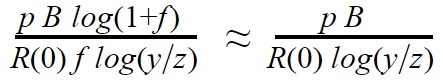. This again fits the 3-factor model, with scale B, neglectedness 1/R(0), and tractability p/log(y/z). However you might properly want to add adjustment factors for the deviation from reality of each assumption and approximation that we have made.

The value from displaced resources is given by:

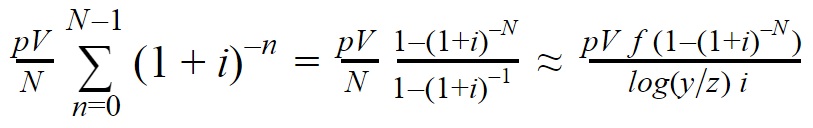 (assuming f and i are both small).

Again if N is large enough this approximates to something simpler, this time pVf/(log(y/z) i). The value from displaced resources unsurprisingly doesn’t depend on the benefit expected, so doesn’t fit with the three-factor model. For problems where the benefit is large but may be far off, the contribution from displaced resources will be quite small and can perhaps be safely ignored. This will be most relevant for problems where a solution is expected fairly quickly, where accounting for the displaced resources could act as a substantial factor in favour of a cause. From examining plausible values, however, I think it will rarely affect the answer by more than a factor of 2, in cases where the problem could be a worthwhile use of resources.

Conclusions

I’ve gone fairly fast in making assumptions where needed to get towards a usable model. I think this was the right way to start: we’ve ended up with a model which isn’t too hard to use, and gives numerical answers to questions we began with no good way to put numbers to. Because of the various modelling assumptions, those numbers won’t be perfect, but I think in most cases the assumptions will have introduced not more than an error factor of perhaps two or three. This makes it a good starting point for this analysis, which may be able to make some meaningful comparisons.

I think that one of the best things to do with the model now is to start applying it and see how it goes in practice. I’ve done a little of this myself (details to follow), but the end method is simple enough that a broader community could valuably use it in making Fermi estimates.

The version I’d use for first-pass Fermi estimates is one of the simplest we saw:

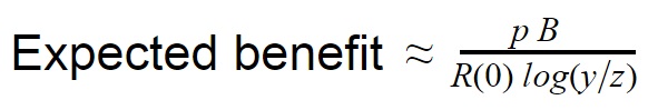
For example, to estimate how valuable extra research into nuclear fusion is, we might estimate that annual spending R(0) = $5B, the annual benefit B = $1000B, and there’s a 50% chance of success (p = 0.5) by the time we’ve spent 100 times as many resources as today (log(y/z) = log(100) = 4.6). Putting these together would give an expected societal benefit of $22 for every dollar spent. This is high enough to suggest that we may be significantly underinvesting in fusion, and that a more careful calculation (with better-researched numbers!) might be justified.

Using the less simplified forms derived above to get a bit of extra accuracy may be useful when you can afford more time and attention to your calculation than a quick back-of-the-envelope job. In a similar vein, I think it could be valuable to try perturbing some of my other assumptions and see what effect that has on the final answer. For example, if the difficulty is not distributed as in the box model but instead in a log-normal distribution, what effect does that have? Or can we get some data which shows how the assumption that other funding is unresponsive to what we do fails?

I hope that we’ll be able to get answers to these questions, and that looking back in a few years this first attempt will seem painfully crude. But in the meantime, I hope these tools will be helpful to people thinking about the value of working on problems of unknown difficulty.